We are often asked how much of a plan’s assets should be allocated to microcap equities. As long-term investors that view the opportunity set through the lens of factors, our answer is usually some version of "probably more than you currently do." Microcap is a very challenging asset class to evaluate. There is little empirical research specific to the intricacies of the space, and common benchmarks cast a shadow on the alpha that is readily apparent in active manager returns and factor spreads. As I have written about previously, true microcap offers substantial opportunity for differentiated alpha generation. This post attempts to provide an alternative framework for approaching and sizing strategic allocations to microcaps.

Optimization Meltdown

Asset allocation typically involves some form of optimization process that requires return, risk, and correlation assumptions. The table below shows common proxies for U.S. equity asset classes. As you move from top to bottom, returns decrease and volatility rises, causing decreasing risk-adjusted return (Sharpe Ratio). While lower return and higher volatility are not enough in and of themselves to eliminate an asset class from inclusion, correlations can. As one can infer from the benchmark statistics below, typical mean-variance optimization will suggest no allocation to the microcap asset class.

A simple test to determine the efficacy of adding an asset class to a portfolio is to look at correlation-adjusted Sharpe ratios.[1] To do this, simply multiply the Sharpe Ratio of an existing portfolio by its correlation with the new asset. The Sharpe of the new asset would then need to be greater than this adjusted Sharpe Ratio to be included. In the table below, both the Russell 2000 and Microcap would fail this test when compared with a 100% Russell 1000 portfolio.

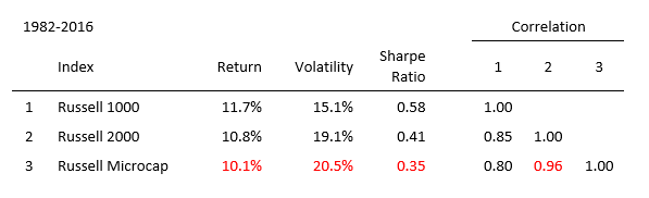
While it would be easy to write off small and microcap as an asset class, a key issue I detailed in a previous post is the poor construction of the commonly used Russell Microcap benchmark.[2] Significant overlap with the Russell 2000® Index, about 88%[3], results in correlation between the indices of 0.96, resulting in little differentiation. This causes microcap as an asset class, defined by Russell, to fail simple tests for strategic inclusion in portfolios. This begs the question of whether cap-weighted benchmarks should always be the de facto measuring stick for asset classes. In my experience researching small and microcap portfolios, it is abundantly clear to that there is ample opportunity to generate return that is distinct from cap-weighted benchmarks.

A Returns-based Approach to Allocation

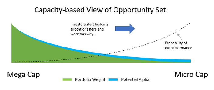
Many practitioners and academics agree that the “market” is an aggregation of stocks weighted by market capitalization. While this is certainly accurate, it represents a capacity-based view of the opportunity set.

Constructing a portfolio, or index, in proportion to market cap weights is unique in that it provides the lowest cost, highest capacity exposure to the market, regardless of investor size. It requires minimal trading beyond dividend reinvestment and investor driven flows because portfolio weights adjust in proportion to changes in market weights as stocks rise and fall. This minimizes ongoing implementation costs.

For active managers, the proposition is that an alternative portfolio exists which will survive ongoing implementation costs required to maintain exposure to its strategy. As the size of the investable portfolio grows, aligning that portfolio more closely with market cap weights becomes a necessity, not an option, because research has shown that implementation costs rise at approximately the square root of assets.[4]. This implicitly concentrates the bulk of investor equity exposure into more competitive portions of the market—large, liquid names. While this is great for maximizing strategy capacity, alpha becomes more scarce as market cap increases. This disadvantages larger investors relative to their smaller counterparts.

The opportunity for alpha can be defined along two dimensions: consistency and magnitude. Consistency relates to how often alpha opportunities exist; base rates, or batting averages, capture this concept. Strategies that win more often than they lose are predisposed to generate persistent outperformance over time. However, if the average loss is greater than the average win, the power of consistency is diminished. Investors seeking persistent and outsized gains relative to some benchmark attempt to identify situations where consistency is in their favor, and the magnitude of wins is greater than that of losses. When properly aligned, consistency and magnitude have a compounding effect over time. A capacity-based view of the opportunity set runs exactly opposite of this concept, favoring allocations where consistency and magnitude are lowest.

The chart below represents a stylized capacity-based view of the equity opportunity set. Notice how the probability of outperformance is inversely related to the largest allocations.

For all but the largest investors, I would argue a returns-based approach is likely more applicable for assessing the opportunity set. The returns-based view begins by disaggregating the effect of market cap to equal weight the opportunity set. This has the effect of pulling allocations away from the largest, most liquid names.

Viewed as a level playing field, investors would begin allocating to asset classes for which the magnitude and consistency of alpha is aligned and highest. Adjustments related to investor risk tolerances, constraints, and costs of implementation could then be made with a greater understanding of the tradeoffs associated with those decisions.

Factor Spreads as a Proxy for Alpha

To evaluate the opportunity for alpha, two breakpoints are established within the U.S. market. The first breakpoint demarcates the difference between Large Stocks, which have a market cap greater than the average across all investable stocks on the U.S. market, and Small Stocks, which have a market cap less than average. The second breakpoint sets the minimum market cap of $200 million for Small Stocks. Stocks below $200 million and greater than $50 million are designated as Microcap Stocks.[5]

Within each particular asset class, factor spreads serve as a decent proxy for the availability of alpha. Factor spread is defined as the return of a portfolio of stocks falling into the highest-ranked decile of a factor minus the return of a portfolio comprised of the lowest-ranked decile of a factor. In the chart below, which shows the results of investing based on a multi-factor value theme within the micro and large stock universes, respectively, this would be the difference between the excess return of decile 1 and decile 10—28.2% for micro and 12.4% for large stocks. [6] Clearly, the microcap portion of the U.S. stock market has significantly wider spreads, more than twice that of Large Stocks, which suggests the opportunity to generate alpha is higher.

There are two key inferences from the chart above. First, stocks ranking in the cheapest decile within the microcap universe deliver on average nearly 3x the excess return of their large counterparts. They also outperform almost 25% more often in rolling three-year periods. Second, the most expensive stocks underperform their large counterparts by 2x, which suggests the benefits of avoiding the most expensive stocks are much greater. This helps explain why passive allocations in small and microcap fair worse in mega and large cap. The most expensive stocks also underperform with greater consistency, 95.4% of the time versus expensive large stocks which underperform only 79.4% of the time. This suggests a relatively greater opportunity for alpha generation and a wide margin for error in stock selection that provides flexibility to accommodate real world constraints.

Practically, this is reflective of how the results for active management have played out over the last decade. The chart below shows the performance of active managers within the micro, small, and large cap competitive universes.[7] The median micro cap manager outperformed the Russell Microcap benchmark by 2.55%—net of fees—while the median large cap manager underperformed the Russell 1000 by -0.46%. Even the 75th percentile manager in the micro cap universe outperformed the Russell Microcap benchmark by 1.21%.

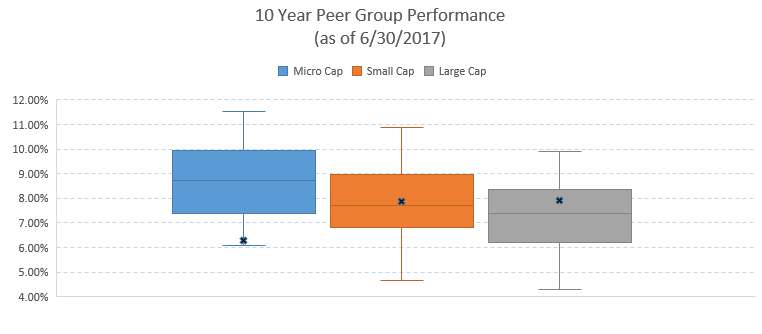
Note: Russell Microcap, Russell 2000, Russell 1000 represented by black dots. Source: PSN

Notice how the performance of the median manager decreases relative to the universe, and how the spread between the top and bottom quartile manager shifts lower. In other words, the magnitude and likelihood of alpha generation is inversely correlated to market cap, benchmark construction, and ultimately, the competitive nature of the space.

Generating Return “Expectations”

One challenge we often face as quantitative investors is the idea of developing return expectations. Frankly, forecasts give a false sense of precision, and should always be taken with a grain of salt. Though I believe that over very long periods, themes like value, momentum, yield, and quality will offer investors superior risk-adjusted return, there is no way to forecast the next year, three years, or even five years with any certainty.

A good bit of the academic literature suggests that the factor themes mentioned above represent risk “premiums.” The concept of premiums is a bit curious because it is suggestive of something that is always available, whereas, factors historically come in and out of favor. A mean-reverting perspective seems a more accurate depiction of the ebb and flow that is inherent in all factors. Since factor timing is a yet unsolved mystery, a reasonable approach seems to be consistent diversified exposure to multiple factor themes.

To illustrate, I created a hypothetical factor-based microcap portfolio. The portfolio is constructed by starting with a Microcap Stocks universe and eliminating stocks falling into the worst decile by our stock selection themes of financial strength, earnings quality, and earnings growth.[8] The portfolio then focusses in on stocks with the strongest combined score by our momentum and value themes. The portfolio is refreshed monthly based on a rolling annual rebalance.

After generating a return stream for this portfolio for the 35 year period from 1982-2016, the portfolio’s return is regressed on the excess return of the highest-ranking decile of the various factor themes to generate exposures, column 1 and 2 in the table below, respectively. I ran the same process for the benchmark in column 4. The contribution to return from factor exposures are in columns 3 and 5 for the portfolio and benchmark, respectively. Column 6 represents the Active Exposure—the difference in exposure for the portfolio and benchmark. Finally, column 7 decomposes the Factor Impact on the portfolio’s excess return. Using the Value line item as an example, the highest-ranked decile of stocks ranked by the value theme outperformed the universe return of 9.0% by an annualized 11.3% excess return. The portfolio had a 0.34 overweight exposure to Value, which contributed annualized excess of 3.9% to return over the full period.

Based on the results of this three-and-a-half-decade study, I make the intellectual leap that factor excess returns, volatility, and correlation in the future will somewhat resemble those of the past. Over reasonable time frames, this has been a decent assumption.[10]

“Expected” return, volatility, and risk-adjusted return (Sharpe) can be found at the bottom of the table. Since absolute returns are incredibly difficult, if at all possible to predict, the more instructive info is likely the excess return, tracking error, and information ratio. The table is suggestive that this factor based portfolio, which demonstrates strong active exposures to value and momentum, should generate excess return of 6.0% over the long-term. For perspective, this level of excess return would be representative of the 5th percentile manager within the microcap manager peer universe over the last 10 years. A key assumption that cannot be emphasized enough is consistent factor exposure throughout the period. For example, if this hypothetical strategy started buying growth stocks without regard to valuation in the 1990’s, this data becomes irrelevant. Discipline to any strategy is key to avoid behavioral pitfalls on a go-forward basis.

I performed similar exercises to generate factor-based portfolios within the large and small stock universes. To provide some diversification of factor exposure across the universe, the large portfolio uses Shareholder Yield as its final selection factor, and the small portfolio uses the Value composite theme. Results for those portfolios are included below.

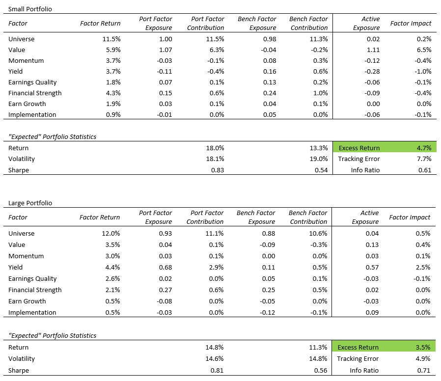
exhibit - expected returns - large, small.PNG

In both cases, factor exposures are about as expected, the small portfolio had strong active value exposure with benchmark-like quality and momentum exposure. The large portfolio had strong active Shareholder Yield exposure, and mostly benchmark or better elsewhere. In both cases, the “expected” excess is on par with top active managers over the previous 10 years as illustrated in the chart above.

Determining Allocations

Finally, having generated expectations for excess return and volatility in micro, small, and large portfolios, we can apply the results in the common mean-variance optimization (MVO) framework to determine overall equity portfolio weights.

The inputs required for MVO are expected returns and covariances. I use the expected returns generated in the analysis above as inputs. The return streams for the portfolios are then used to generate a covariance matrix. Implicit is the assumption that covariances are stationary over time. We know this not to be the case in the short-term, so care should be taken to interpret the results only in the context of long-term strategic, not tactical, decisions. The correlation matrices below demonstrate the differentiated return profile that can be generated with carefully constructed factor portfolios as distinct from relying on market cap weighted benchmarks in asset allocation. Notice the decrease in correlation between the Micro and Small portfolios and the Russell 2000 and Russell Micro benchmarks.

Armed with expected returns and covariances, I apply very few constraints to the overall portfolio optimization. The portfolio must be fully invested at all times, and shorting is not allowed. Other than that, no constraints are needed to “force” the optimization into reasonable results. The objective is maximizing risk-adjusted return via the Sharpe Ratio.

The table below displays the results of the MVO process. Weighting to the micro and small portfolios are much greater than most allocators are probably used to at a combined 57% of the equity portfolio. The lower portion of the table includes summary statistics for our hypothetical optimization of the micro, small, and large factor portfolios as compared to the cap-weighted benchmarks at the optimization weights. Contrary to what might be commonly expected, the increased allocations do not result in dramatic increases in volatility. Volatility actually decreases by 1%. With 4.5% annualized excess return and 1% lower volatility, the Sharpe ratio increases dramatically.

As a comparator, I ran a parallel comparison which uses expected returns and volatility for the Russell benchmarks as proxies for cap-weighted portfolios. The results are much more in-line with typical investor allocations, though still probably higher on small cap than expected.

Thus far, we have not considered the risk tolerance of the allocator. While one set of investors may be perfectly comfortable with significant micro and small cap exposure, certain investors probably need to adjust portfolios to their risk preferences.

It turns out that there is a relatively simple way to scale portfolio returns based on volatility. This entails incorporating a penalty factor for portfolios that adjusts based on an investor’s risk aversion. Risk averse investors would incorporate a greater penalty in determining their appropriate policy portfolio. Less risk averse investors would incorporate lower penalties. Risk aversion could be modeled to incorporate any number of different characteristics—investment horizon, sensitivity to absolute and/or relative drawdowns, liquidity needs, etc. For this post, I demonstrate an example based on volatility.[11]

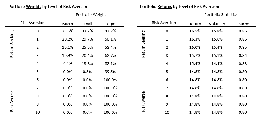
In the table below, a Risk Aversion score of 0 represents the utility of each portfolio for a return-seeking investor, effectively the results we determined in the MVO analysis above. We then apply successively increasing risk penalties based on the volatility of each portfolio. Because the micro and small portfolios are more volatile than large cap, returns decrease to the point at which the utility of the micro and small portfolio are close to indifferent with large by the time a risk aversion score of 5 is reached. Think of the returns below as a proxy for how the investor feels about the level of return given the volatility required to achieve that return. A highly risk averse investor with a score of 10 significantly prefers the large cap portfolio rather than small or microcap.

These utility-adjusted returns can then be used as expected return inputs into additional MVO analysis which adjusts allocations of the total equity portfolio for individual risk aversion. The table below displays these results at each level of risk aversion. As risk aversion increases, the optimal weight dials down exposure to the micro and small strategies in favor of the lower volatility large strategy. In my experience, most investors fall in the 3 to 6 range.

Conclusion

It would behoove of investors to recognize traditional indexes for what they are, factor-based strategies predicated on one factor, market cap. Though market cap has everything to do with low cost implementation, high capacity, and cheap beta exposure, it has little to do with optimal investor allocations for all but the largest plans.

Breaking from the capacity-based, cap-weighted perspective allows investors and allocators to focus on asset classes in which "edges" are apparent and hidden within traditional benchmarks. Allocators should view portfolios through the lens of consistent factor exposures over multiple market cycles. Doing so allows for reasonable "expected" excess returns that are otherwise overshadowed by cap-weighted indexes when used as proxies for asset class returns. Further, poor benchmark construction can, in and of itself, actually eliminate entire asset classes from consideration.

Using long-run factor excess, correlation, and risk aversion inputs in traditional MVO analysis yields surprising results that suggest volatility reduction and return enhancement through inclusion of micro and small cap stocks in equity asset allocation.

---

[1] See appendix for more detail and references.

[2] “Microcaps — Factor Spreads, Structural Biases, and the Institutional Imperative”. August 2017.

[3] As of 12/31/2016

[4] “Asset Growth and Its Impact on Expected Alpha.” Ronald N. Kahn.

[5] Market cap breakpoints are adjusted for inflation historically.

[6] The value theme is defined as an equal-weighted score of ranking based on price to sales, price to earnings, ebitda-to-ev, free cash flow-to-ev, and shareholder yield. Shareholder yield is the combination of share buybacks and dividend yield.

[7] PSN

[8] See Appendix for Factor Theme descriptions.

[9] See Appendix for Factor Theme descriptions.

[10] See Factor Correlations in Appendix

[11] For a detailed explanation of our approximation of risk aversion, see the appendix and Bodie, Kane, and Marcus (2004, p. 168).

Appendix

Decision to Add the Asset Class

For an investor deciding to gain exposure to an asset class, the decision itself can be addressed through common frameworks that seek to balance risk-return tradeoffs. Blume (1984) and Elton, Gruber, and Rentzler (1987) suggest that the decision to add an asset class to an existing portfolio can be determined by comparing the Sharpe ratio of the new asset class with the correlation adjusted Sharpe ratio of the existing portfolio. The correlation adjustment is important as it incorporates the benefits of risk reduction when evaluating the new asset.

Factor Theme Descriptions

Universe - The market factor is an equal-weighted selection universe for the portfolio.

Value - The excess return of the highest-ranking decile of a Value Composite relative to the selection universe. The Value Composite consists of underlying constituents such as price relative to sales, earnings and cash flows.

Momentum - The excess return of the highest-ranking decile of a Momentum Composite relative to the selection universe. Momentum consists of four underlying constituents—3-month, 6-month, and 9-month momentum, and twelve month volatility.

Yield - The excess return of the highest-ranking decile of Shareholder Yield relative to the selection universe.

Earnings Quality - The excess return of the highest-ranking decile of an Earnings Quality Composite relative to the selection universe. The composite consists of several underlying constituents, which measure the conservatism of accounting choices through accruals.

Financial Strength - The excess return of the highest-ranking decile of a Financial Strength Composite relative to the selection universe. The composite consists of multiple underlying constituents, which assess balance sheet leverage and strength.

Earnings Growth - The excess return of the highest-ranking decile of an Earnings Growth Composite relative to the selection universe. The composite consists of multiple underlying constituents, which measure the consistency of earnings and profitability.

Implementation – A proxy for the cost of implementation is measured using two factors that historically correlate with the cost of trading, such as dollar volume and market cap.

Factor Correlations

The table below includes summary stats for the rolling 36-month correlation of the highest-ranked decile of six factor themes encompassing value, momentum, yield, and quality relative to the microcap universe. Correlations are on average above 0.9, with deviations within reasonable bounds.

Risk Aversion

Risk aversion can be proxied through utility theory. Practically, the return of a portfolio can be adjusted through a penalty factor for increased volatility. Risk averse investors would incorporate a greater penalty in determining their appropriate policy portfolio. Less risk averse investors would incorporate lower penalties based on increases in risk. Risk aversion could be modeled to incorporate a number of different characteristics—investment horizon, sensitivity to absolute and/or relative drawdowns, liquidity needs, etc.

Bode Kane, and Marcus (2004) outline a simple equation for modeling risk aversion.